GeoMesa Kafka Streams Quick Start
This tutorial demonstrates using Kafka Streams with GeoMesa. It will walk-through reading from and writing to a GeoMesa-Kafka topic and using Kafka Streams to process data.
About this Tutorial
This tutorial utilizes the same components as the GeoMesa Kafka Quick Start and can be viewed as an expansion of it. Here we will:
Establishes a new (static) SimpleFeatureType
Prepares the Kafka topic to write this type of data
Creates a few thousand example SimpleFeatures
Writes these SimpleFeatures to the Kafka topic
Consume these features from the topic using Kafka Streams
Process the consumed features
Write the result back to the same Kafka topic
Visualize the changing data in GeoServer (optional)
The quick start operates by simultaneously querying and writing several thousand feature updates. The data contains location information for two entities. A unique feature identifier is used for each entity. Updates for an entity will re-use the entity’s feature identifier such that there will only be one live feature for each entity.
The Kafka Streams topology will be configured to look for instances when the two entities are withing a distance threshold of each other. These proximity events are written back to the same topic with a unique feature identifier so that they persist in the layer.
The data used is a simulated drive between Charlottesville and Richmond Virginia, following the I64 interstate.
Background
Apache Kafka is “publish-subscribe messaging rethought as a distributed commit log.”
In the context of GeoMesa, Kafka is a useful tool for working with streams of geospatial data. Interaction with Kafka in GeoMesa occurs through the KafkaDataStore which implements the GeoTools DataStore interface.
Additionally, GeoMesa configures a Kafka Streams topology to read, process and write data to the topic. More information about Kafka Streams can be found in the official documentation.
Prerequisites
Before you begin, you must have the following installed and configured:
Ensure your Kafka and Zookeeper instances are running. You can use Kafka’s quickstart to get Kafka/Zookeeper instances up and running quickly.
Configure GeoServer (optional)
You can use GeoServer to access and visualize the data stored in GeoMesa. In order to use GeoServer, download and install version 2.27.2. Then follow the instructions in Installing GeoMesa Kafka in GeoServer to enable GeoMesa.
Download and Build the Tutorial
Pick a reasonable directory on your machine, and run:
$ git clone https://github.com/geomesa/geomesa-tutorials.git
$ cd geomesa-tutorials
Warning
Make sure that you download or checkout the version of the tutorials project that corresponds to your GeoMesa version. See About Tutorial Versions for more details.
To ensure that the quick start works with your environment, modify the pom.xml
to set the appropriate versions for Kafka, Zookeeper, etc.
For ease of use, the project builds a bundled artifact that contains all the required dependencies in a single JAR. To build, run:
$ mvn clean install -pl geomesa-tutorials-kafka/geomesa-tutorials-kafka-streams-quickstart -am
Running the Tutorial
On the command line, run:
$ java -cp geomesa-tutorials-kafka/geomesa-tutorials-kafka-streams-quickstart/target/geomesa-tutorials-kafka-streams-quickstart-5.4.0.jar \
    org.geomesa.example.kafka.KafkaStreamsQuickStart \
    --kafka.brokers <brokers>                 \
    --kafka.zookeepers <zookeepers>
where you provide the following arguments:
<brokers>your Kafka broker instances, comma separated. For a local install, this would belocalhost:9092<zookeepers>your Zookeeper nodes, comma separated. For a local install, this would belocalhost:2181
Optionally, you can also specify that the quick start should delete its data upon completion. Use the
--cleanup flag when you run to enable this behavior.
Once run, the quick start will create the Kafka topic, then pause and prompt you to register the layer in GeoServer. If you do not want to use GeoServer, you can skip this step. Otherwise, follow the instructions in the next section before returning here.
Once you continue, the tutorial should run for approximately thirty seconds. You should see the following output:
Loading datastore

Loading datastore

Creating schema: entityId:String,dtg:Date,geom:Point

Generating test data

Configuring Streams Topology
Feature type created - register the layer 'cvilleric-quickstart' in geoserver with bounds: MinX[-78.4696824929457] MinY[37.532442090296044] MaxX[-77.42668269989638] MaxY[38.03920921521279]
Press <enter> to continue


Writing features to Kafka... refresh GeoServer layer preview to see changes
Current consumer state:
a=a|2022-09-21T21:03:02.675Z|POINT (-78.2742794712714 37.995618168053184)
b=b|2022-09-21T21:03:02.675Z|POINT (-77.56747216770198 37.6305975318267)
Current consumer state:
a=a|2022-09-21T21:28:02.675Z|POINT (-78.01751112645616 37.872800086051654)
b=b|2022-09-21T21:28:02.675Z|POINT (-77.87883454073382 37.772794168668476)
Current consumer state:
b=b|2022-09-21T21:53:02.675Z|POINT (-78.14780655790103 37.95424382536054)
a=a|2022-09-21T21:53:02.675Z|POINT (-77.711327871061 37.694257161353974)
proximity0ab51dd3-2e48-4827-9388-c76c7f95279b=proximity-a-b|2022-09-21T21:35:02.675Z|POINT (-77.94037514437152 37.81389651562376)
proximity911fd4dd-40c8-4336-90aa-0315e4d896b5=proximity-b-a|2022-09-21T21:33:02.675Z|POINT (-77.94037514437152 37.81389651562376)
proximity70a19c33-8d77-4539-b2a0-5d4f0abfcd9a=proximity-a-b|2022-09-21T21:33:02.675Z|POINT (-77.96397858370257 37.828337948614255)
proximityaef4c251-9edb-4d96-8a1a-65da5a40c11d=proximity-b-a|2022-09-21T21:34:02.675Z|POINT (-77.95393639315081 37.82182948351288)
proximity3025cd2b-699a-4625-9760-2781acf98edf=proximity-a-b|2022-09-21T21:34:02.675Z|POINT (-77.95393639315081 37.82182948351288)
proximity0eb6874d-19c1-4c55-887f-ff8e50455662=proximity-b-a|2022-09-21T21:35:02.675Z|POINT (-77.96397858370257 37.828337948614255)
Current consumer state:
b=b|2022-09-21T22:18:02.675Z|POINT (-78.40589688999782 38.018104630123695)
a=a|2022-09-21T22:18:02.675Z|POINT (-77.46880947199425 37.579440835126896)
proximity0ab51dd3-2e48-4827-9388-c76c7f95279b=proximity-a-b|2022-09-21T21:35:02.675Z|POINT (-77.94037514437152 37.81389651562376)
proximity911fd4dd-40c8-4336-90aa-0315e4d896b5=proximity-b-a|2022-09-21T21:33:02.675Z|POINT (-77.94037514437152 37.81389651562376)
proximity70a19c33-8d77-4539-b2a0-5d4f0abfcd9a=proximity-a-b|2022-09-21T21:33:02.675Z|POINT (-77.96397858370257 37.828337948614255)
proximityaef4c251-9edb-4d96-8a1a-65da5a40c11d=proximity-b-a|2022-09-21T21:34:02.675Z|POINT (-77.95393639315081 37.82182948351288)
proximity3025cd2b-699a-4625-9760-2781acf98edf=proximity-a-b|2022-09-21T21:34:02.675Z|POINT (-77.95393639315081 37.82182948351288)
proximity0eb6874d-19c1-4c55-887f-ff8e50455662=proximity-b-a|2022-09-21T21:35:02.675Z|POINT (-77.96397858370257 37.828337948614255)


Done
Visualize Data With GeoServer (optional)
You can use GeoServer to access and visualize the data stored in GeoMesa. In order to use GeoServer, download and install version 2.27.2. Then follow the instructions in Installing GeoMesa Kafka in GeoServer to enable GeoMesa.
Register the GeoMesa Store with GeoServer
Log into GeoServer using your user and password credentials. Click
“Stores” and “Add new Store”. Select the Kafka (GeoMesa) vector data
source, and fill in the required parameters.
Basic store info:
workspacethis is dependent upon your GeoServer installationdata source namepick a sensible name, such asgeomesa_quick_startdescriptionthis is strictly decorative;GeoMesa quick start
Connection parameters:
these are the same parameter values that you supplied on the command line when you ran the tutorial; they describe how to connect to the Kafka instance where your data resides
Click “Save”, and GeoServer will search Zookeeper for any GeoMesa-managed feature types.
Publish the Layer
If you have already run the command to start the tutorial, then GeoServer should recognize the
cvilleric-quickstart feature type, and should present that as a layer that can be published. Click on the
“Publish” link. If not, then run the tutorial as described above in Running the Tutorial. When
the tutorial pauses, go to “Layers” and “Add new Layer”. Select the GeoMesa Kafka store you just
created, and then click “publish” on the cvilleric-quickstart layer.
You will be taken to the Edit Layer screen. You will need to enter values for the data bounding boxes. For this demo, use the values MinX: -78.46969, MinY: 37.53245, MaxX: -77.42669, MaxY: 38.03921.
Click on the “Save” button when you are done.
Style the Layer (optional)
To better visualize the interaction of input data and data generated by the Kafka Stream topology it can be helpful to apply some simple styling rules. To do this first create a new style.
Click “Styles” and “Add a new style”. Give it a reasonable name and set the Format to CSS. Insert the following CSS into the editor window.
* {
    mark: symbol(circle);
    mark-size: 9px;
    fill: #1e8003;
}

[entityId = 'a'] :mark {
    fill: #AD0000;
}

[entityId = 'b'] :mark {
    fill: #001AAD;
}
Click “Submit” to save the style. Next the style must be added to the layer and set as default. Under “Layers” select the layer you created. On the “Publishing” tab, under “WMS Setting” and “Layer Settings” set the “Default Style” to the style you created. At the bottom of the page click “Save” to proceed.
Take a Look
Click on the “Layer Preview” link in the left-hand gutter. If you don’t
see the quick-start layer on the first page of results, enter the name
of the layer you just created into the search box, and press
<Enter>.
At first, there will be no data displayed. Once you have reached this point, return to the quick start console and hit “<enter>” to continue the tutorial. As the data is updated in Kafka, you can refresh the layer preview page to see the feature moving around.
What’s Happening in GeoServer
The layer preview of GeoServer uses the KafkaFeatureStore to show a
real time view of the current state of the data stream. There are two
SimpleFeatures being updated over time in Kafka which is
reflected in the GeoServer display.
As you refresh the page, you should see the SimpleFeatures move around.
When the two points (red and blue points below) are close to each other you will see SimpleFeatures representing the
proximity events (grey points below) added to the data stream. These features will remain where they are because there
are no updates being sent with the same feature IDs.
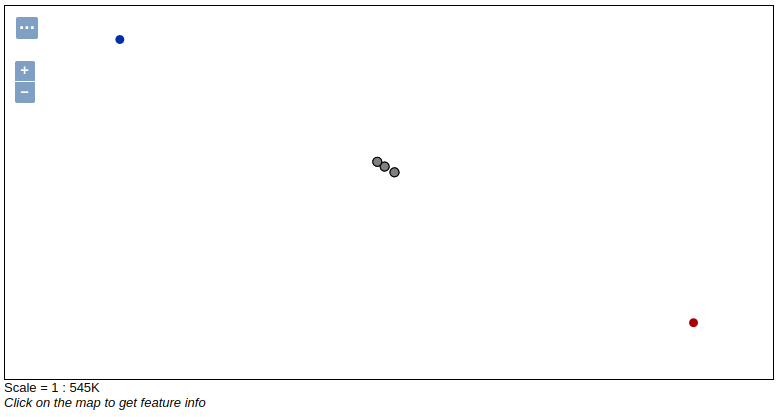
Visualizing quick-start data with GeoServer
Looking at the Code
The source code is meant to be accessible for this tutorial. The logic is contained in
the generic org.geomesa.example.quickstart.GeoMesaQuickStart in the geomesa-quickstart-common module,
and the Kafka-Streams specific org.geomesa.example.kafka.KafkaStreamsQuickStart in the
geomesa-quickstart-kafka-streams module. Some relevant methods are:
createDataStoreoverridden in theKafkaQuickStartto use the input configuration to get a pair of datastore instances, one for writing and one for reading data. Additionally, theGeoMesaStreamsBuilderis used to create the Kafka Streams topology builder.createSchemacreate the schema in the datastore, as a pre-requisite to writing datawriteFeaturesoverridden in theKafkaQuickStartto simultaneously write and read features from Kafka as well as setup and run the streams topologyqueryFeaturesnot used in this tutorialcleanupdelete the sample data and dispose of the datastore instance
Code for parsing the data into GeoTools SimpleFeatures is contained in org.geomesa.example.data.CvilleRICData:
getSimpleFeatureTypecreates theSimpleFeatureTyperepresenting the datagetTestDataparses an embedded CSV file to createSimpleFeatureobjectsgetTestQueriesnot used in this tutorial
Streams Topology
The code in setupStreams uses the GeoMesa Kafka Streams integration to build the Kafka Streams topology. The
GeoMesaStreamsBuilder class wraps an internal Kafka StreamsBuilder instance. This allows GeoMesa to provide the
Kafka Serde when reading and writing data to the underlying Kafka topic and provide the TimestampExtractor
appropriate to the SimpleFeatureType. Additionally, GeoMesa is able to resolve the correct Kafka topic for a given
TypeName.
The quickstart topology reads data from the quickstart topic into a KStream, leveraging the Serde and
TimestampExtractor from GeoMesa.
KStream<String, GeoMesaMessage> input = builder.stream(typeName);
Next the input stream is filtered to remove any messages that are not updates to our two entities. Failure to do this
step would allow the proximity messages we write later to be pickup up and processed by the topology. After filtering
the data is re-keyed. The GeoPartitioner class is a KeyValueMapper that is used to select a new key for each
record. The new key is determined by utilizing a GeoMesa Z2SFC to determine which geospatial Z-Bin a given record
is contained in. More info on Z2 curves and indexing can be found in the Index Overview. Changing the record keys
will cause Kafka Stream to repartition the data stream. This will create an intermediate topic but will ensure that data
is co-located with other data that is spatially proximal.
KStream<String, GeoMesaMessage> geoPartioned = input
    .filter((k, v) -> !Objects.equals(getFID(v), "") && !getFID(v).startsWith(proximityId))
    .selectKey(new GeoPartitioner(numbits, defaultGeomIndex));
To find if a point is in proximity of another requires computing the distance to every other point. To find all proximities in a set of points requires the cartesian product of all points. This can be a very expensive operation so reducing the number of points that need to be compared is important. Spatially partitioning the data allows us to reduce the number of comparisons by excluding spatial regions. Only the cartesian product of records sharing the same Z-Bin need to be evaluated (this tutorial ignores the issue with Z-Bin boundaries).
The quickstart next uses the GeoPartitioned KStream to perform a self join using the, now spatial, keys. This allows
us to create a Proximity object for each comparison that needs to be evaluated.
A self join will by its nature join a record to itself. The filter step first removes these and then performs the actual
proximity calculation and threshold check. Finally we convert the Proximity events into GeoMesaMessage and set
a key that indicates it’s a proximity message (use in the previous filter step).
KStream<String, GeoMesaMessage> proximities = geoPartioned
    .join(geoPartioned,
        (left, right) -> new Proximity(left, right, defaultGeomIndex),
        JoinWindows.of(Duration.ofMinutes(2)),
        StreamJoined.with(Serdes.String(), serde, serde))
    .filter((k, v) -> v.areDifferent() && v.getDistance() < proximityDistanceMeters)
    .mapValues(Proximity::toGeoMesaMessage)
    .selectKey((k, v) -> proximityId + UUID.randomUUID());
Lastly the GeoMesaStreamsBuilder is used again to configure the target topic from the provided TypeName and handle
the Serde for us.
builder.to(typeName, proximities);