GeoMesa Spark: Aggregating and Visualizing Data
This tutorial will show you how to:
- Use GeoMesa with Apache Spark in Scala.
- Calculate aggregate statistics using a covering set of polygons.
- Create a new simple feature type to represent this aggregation.
- Use Jupyter and Leaflet to visualize the result.
The end of the tutorial provides a link to a downloadable Jupyter notebook with all the necessary code.
Background
Apache Spark is a “fast and general engine for large-scale data processing”. Spark presents an abstraction called a Resilient Distributed Dataset (RDD) that facilitates expressing transformations, filters, and aggregations, and efficiently executes the computation across a distributed set of resources. Spark manages the lineage of a block of transformed data so that if a node goes down, Spark can restart the computation for just the missing blocks.
Jupyter Notebook is an interactive web interface for a kernel, which is an environment for running the code of a language. Jupyter allows you quickly prototype by writing code in runnable cells, computing a final result as you go. Visualization of data is also easily done through integration of Jupyter cell “magics” (special directives for functionality outside of the kernel) to create JavaScript and HTML outputs.
Here, we will combine these two services to demonstrate an operation we are naming “Shallow Join”. This operation is a means of imposing a small, covering set of geospatial data onto a much larger set of data. We essentially perform an inner join with the geospatial predicate, then aggregate over the result. All of this is done in a distributed fashion using Spark.
In our example, GDELT data has point geometries for each event, but we do not directly know in which country it took place. We “join” this geometry against the polygons of the covering set in order to calculate statistics for a geographical region. However, the example is general enough to support statistics for any data set with numerical fields or other non-point geometries such as LineStrings or polygons.
Prerequisites
Warning
You will need access to a Hadoop 2.2 or better installation with Yarn as well as an Accumulo 1.7 or 1.8 database.
You will need to have ingested GDELT data using GeoMesa. Instructions are available in Map-Reduce Ingest of GDELT.
You will need to have ingested a shapefile of polygons outlining your regions of choice. In this tutorial we use this shapefile of countries.
You will also need:
- a Spark 2.0.0 or later distribution
- Accumulo user credentials with appropriate permissions to query your data
- Java JDK 8
- a Jupyter Notebook server with the Apache Toree Scala kernel installed
Set Up Tutorial Code
Clone the geomesa-tutorials project, and go into the geomesa-examples-spark directory:
$ git clone https://github.com/geomesa/geomesa-tutorials.git $ cd geomesa-tutorials/geomesa-examples-spark
Note
The code in this tutorial is written in Scala.
Create RDDs
The code described below is found in the com.example.geomesa.spark.ShallowJoin class
in the src/main/scala directory.
First, set up the parameters and initialize each of the desired data stores.
val gdeltDsParams = Map(
  "instanceId" -> "instance",
  "zookeepers" -> "zoo1,zoo2,zoo3",
  "user"       -> "user",
  "password"   -> "*****",
  "auths"      -> "USER,ADMIN",
  "tableName"  -> "geomesa_catalog")

val countriesDsParams = Map(
  "instanceId" -> "instance",
  "zookeepers" -> "zoo1,zoo2,zoo3",
  "user"       -> "user",
  "password"   -> "*****",
  "auths"      -> "USER,ADMIN",
  "tableName"  -> "countries_catalog")

val gdeltDs = DataStoreFinder.getDataStore(gdeltDsParams)
val countriesDs = DataStoreFinder.getDataStore(countriesDsParams)
Next, initialize a SparkContext and get the SpatialRDDProvider for
each data store:
val conf = new SparkConf().setAppName("testSpark")
val sc = SparkContext.getOrCreate(conf)

val rddProviderCountries = GeoMesaSpark(countriesDsParams)
val rddProviderGdelt     = GeoMesaSpark(gdeltDsParams)
Now we can initialize RDDs for each of the two sources.
val countriesRdd: RDD[SimpleFeature] = rddProviderCountries.rdd(new Configuration(), sc, countriesDsParams, new Query("states"))
val gdeltRdd: RDD[SimpleFeature] = rddProviderGdelt.rdd(new Configuration(), sc, gdeltDsParams, new Query("gdelt"))
Grouping by polygons
To perform our shallow join, we send our smaller data set, countries, to each of the partitions of the larger data set, GDELT events. This is accomplished through a Spark broadcast, which serializes the desired data and sends it to each of the nodes in the cluster. This way it is only copied once per task. Note also that we collect the countries RDD into an Array before broadcasting. Spark does not allow broadcasting of RDDs, and due to the small size of the data set, we can safely collect data onto the driver node without a risk of running out of memory.
val broadcastedRegions = sc.broadcast(countriesRdd.collect)
With the covering set available on each partition, we can iterate over the GDELT events and key them by the region they
were contained in. In mapPartitions, iter is an iterator to all the elements (in this case Simple Features) on
the partition. Here we transform each iterator and store the result into a new RDD.
val keyedData = gdeltRdd.mapPartitions { iter =>
    import org.locationtech.geomesa.utils.geotools.Conversions._

    iter.flatMap { sf =>
        // Iterate over regions until a match is found
        val it = broadcastedRegions.value.iterator
        var container: Option[String] = None
        while (it.hasNext) {
          val cover = it.next()
          // If the cover's polygon contains the feature,
          // or in the case of non-point geoms, if they intersect, set the container
          if (cover.geometry.intersects(sf.geometry)) {
            container = Some(cover.getAttribute(key).asInstanceOf[String])
          }
        }
        // return the found country as the key
        if (container.isDefined) {
          Some(container.get, sf)
        } else {
          None
        }
    }
}
Our new RDD is now of type RDD[(String, SimpleFeature)] and can be used for a Spark reduceByKey operation, but
first, we need to create a simple feature type to represent the aggregated data.
Creating a New Simple Feature Type
We first loop through the types of a sample feature from the GDELT RDD to decide what fields can be aggregated.
val countableTypes = Seq("Integer", "Long", "Double")
val typeNames = gdeltRdd.first.getType.getTypes.toIndexedSeq.map{t => t.getBinding.getSimpleName.toString}
val countableIndices = typeNames.indices.flatMap { index =>
    val featureType = typeNames(index)
    // Only grab countable types, skipping the ID field
    if ((countableTypes contains featureType) && index != 0) {
        Some(index, featureType)
    } else {
        None
    }
}.toArray
val countable = sc.broadcast(countableIndices)
With these fields, we can create a Simple Feature Type to store their averages and totals, prefixing each one with “total_” and “avg_”. Of course, it may not make sense to aggregate ID fields or fields that are already an average, should they appear, but this approach makes it easy if the fields are not known ahead of time.
val sftBuilder = new SftBuilder()
sftBuilder.stringType("country")
sftBuilder.multiPolygon("geom")
sftBuilder.intType("count")
val featureProperties = gdeltRdd.first.getProperties.toSeq
countableIndices.foreach { case (index, clazz) => {
    val featureName = featureProperties.apply(index).getName
    clazz match {
        case "Integer" => sftBuilder.intType("total_" + featureName)
        case "Long" => sftBuilder.longType("total_" + featureName)
        case "Double" => sftBuilder.doubleType("total_" + featureName)
    }
    sftBuilder.doubleType("avg_"+featureProperties.apply(index).getName)
    }
}
val coverSft = SimpleFeatureTypes.createType("aggregate",sftBuilder.getSpec)
Aggregating by Key
To begin aggregating we first send our new Simple Feature Type to each of the executors so that they can create and serialize Simple Features of that type.
GeoMesaSpark.register(Seq(coverSft))

val newSfts = sc.broadcast(GeoMesaSparkKryoRegistrator.typeCache.values.map { sft =>
    (sft.getTypeName, SimpleFeatureTypes.encodeType(sft))
}.toArray)

keyedData.foreachPartition { iter =>
    newSfts.value.foreach { case (name, spec) =>
        val newSft = SimpleFeatureTypes.createType(name, spec)
        GeoMesaSparkKryoRegistrator.putType(newSft)
    }
}
Now we can apply a reduceByKey operation to the keyed RDD. This Spark operation will take pairs of RDD elements of
the same key, apply the given function, and replace them with the result. Here, we have three cases for reduction.
- The two Simple Features have not been aggregated into one of a new type.
- The two Simple Features have both been aggregated into one of a new type.
- One of the Simple Features has been aggregated (but not both).
For the sake of brevity, we will only show the first case, with the other two following similar patterns.
// Grab each feature's properties
val featurePropertiesA = featureA.getProperties.toSeq
val featurePropertiesB = featureB.getProperties.toSeq
// Create a new aggregate feature to hold the result
val featureFields = Seq("empty", featureA.geometry) ++ Seq.fill(aggregateSft.getTypes.size-2)("0")
val aggregateFeature = ScalaSimpleFeatureFactory.buildFeature(aggregateSft, featureFields, featureA.getID)

// Loop over the countable properties and sum them for both gdelt simple features
countable.value.foreach { case (index, clazz) =>
    val propA = featurePropertiesA(index)
    val propB = featurePropertiesB(index)
    val valA = if (propA == null) 0 else propA.getValue
    val valB = if (propB == null) 0 else propB.getValue

    val sum  = (valA, valB) match {
        case (a: Integer, b: Integer) => a + b
        case (a: java.lang.Long, b: java.lang.Long) => a + b
        case (a: java.lang.Double, b: java.lang.Double) => a + b
        case _ => throw new Exception("Couldn't match countable type.")
    }
    // Set the total
    if( propA != null)
        aggregateFeature.setAttribute("total_"+ propA.getName.toString, sum)

}
aggregateFeature.setAttribute("count", new Integer(2))
aggregateFeature
Spark also provides a combineByKey operation that also divides nicely into these three cases, but is slightly more
logically complex.
With the totals and counts calculated, we can now compute the averages for each field. Also, while iterating, we can add the country name and geometry to each feature. To do that, we first broadcast a map of name to geometry.
val countryMap: scala.collection.Map[String, Geometry] =
    countriesRdd.map { sf =>
        (sf.getAttribute("NAME").asInstanceOf[String] -> sf.getAttribute("the_geom").asInstanceOf[Geometry])
    }.collectAsMap

val broadcastedCountryMap = sc.broadcast(countryMap)
Then we can transform the aggregate RDD into one with averages and geometries added.
val averaged = aggregate.mapPartitions { iter =>
    import org.locationtech.geomesa.utils.geotools.Conversions.RichSimpleFeature

    iter.flatMap { case (countryName, sf) =>
        if (sf.getType.getTypeName == "aggregate") {
            sf.getProperties.foreach { prop =>
                val name = prop.getName.toString
                if (name.startsWith("total_")) {
                    val count = sf.get[Integer]("count")
                    val avg = (prop.getValue) match {
                            case (a: Integer) => a / count
                            case (a: java.lang.Long) => a / count
                            case (a: java.lang.Double) => a / count
                            case _ => throw new Exception(s"couldn't match $name")
                    }

                    sf.setAttribute("avg_" + name.substring(6), avg)
                }
            }
            sf.setAttribute("country", countryName)
            sf.setDefaultGeometry(broadcastedCountryMap.value.getOrElse(countryName,null))
            Some(sf)
        } else {
            None
        }
    }
}
Visualization
At this point, we have created a new Simple Feature Type representing aggregated data and an RDD of Simple Features of this type. The above code can all be compiled and submitted as a Spark job, but if placed into a Jupyter Notebook, the RDD can be kept in memory and even quickly tweaked while continuously updating visualizations.
With a Jupyter notebook server running with the Apache Toree kernel (see Deploying GeoMesa Spark with Jupyter Notebook), create a notebook with the above code. The next section highlights how to create visualizations with the aggregated data.
While there are many ways to visualize data from an RDD, here we choose to demonstrate the use of Leaflet, a JavaScript
library for creating interactive maps, for easy integration of the map image with Jupyter Notebook. To use, either
install it through Jupyter’s nbextensions tool, or place the following HTML in your notebook to import it properly.
Note that we preface it with %%HTML, a Jupyter cell magic, indicating that the cell should be interpreted as HTML.
%%HTML
<link rel="stylesheet" href="http://cdn.leafletjs.com/leaflet/v0.7.7/leaflet.css" />
<script src="http://cdn.leafletjs.com/leaflet/v0.7.7/leaflet.js"></script>
The problem of getting data from an RDD in the Scala Kernel to client-side JavaScript can also be solved in many ways.
One option is to save the RDD to a GeoMesa schema and use the GeoServer Manager API to publish a WMS layer. Leaflet
is capable of then reading a WMS layer into its map via HTTP. A more direct route, however, is to export the RDD as GeoJSON.
To do this, use Toree’s AddDeps magic to add the GeoTool GeoJSON dependency on the fly.
%AddDeps org.geotools gt-geojson 14.1 --transitive --repository http://download.osgeo.org/webdav/geotools
We can then transform the RDD of Simple Features to an RDD of strings, collect those strings from each partition, join them, and write them to a file.
import org.geotools.geojson.feature.FeatureJSON
import java.io.StringWriter
val geoJsonWriters = averaged.mapPartitions{ iter =>
    val featureJson = new FeatureJSON()
    val strRep = iter.map{ sf =>
        featureJson.toString(sf)
    }
    // Join all the features on this partition
    Iterator(strRep.mkString(","))
}
// Collect these strings and joing them into a JSON array
val geoJsonString = geoJsonWriters.collect.mkString("[",",","]")

// Write to file
In order to modify the DOM of the HTML document from within a Jupyter cell, we must set up a Mutation Observer to correctly
respond to asynchronous changes. We attach the observer to element, which refers to the cell from which the JavaScript
code is run. Within this observer, we instantiate a new Leaflet map, and add a base layer from OSM.
(new MutationObserver(function() {

    // Initialize the map
    var map = L.map('map').setView([35.4746,-44.7022],3);
    // Add the base layer
    L.tileLayer("http://{s}.tile.osm.org/{z}/{x}/{y}.png").addTo(map);

    this.disconnect()
})).observe(element[0], {childList: true})
Inside the Leaflet we create a tile layer from the GeoJSON file we created. There are further options of creating a layer from an image file or from a GeoServer WMS layer.
var rawFile = new XMLHttpRequest();
rawFile.onreadystatechange = function () {
    if(rawFile.readyState === 4) {
        if(rawFile.status === 200 || rawFile.status == 0) {
            var allText = rawFile.response;
            var gdeltJson = JSON.parse(allText)
            L.geoJson(gdeltJson).addTo(map);
            // Css override
            $('svg').css("max-width","none")
        }
    }
}
rawFile.open("GET", "aggregateGdelt.json", false);
rawFile.send()
There are many opportunities here to style these layers such as coloring polygons by attributes. Here we color each country’s polygon by its average Goldstein scale, indicating how events are contributing to the stability of a country during that time range.
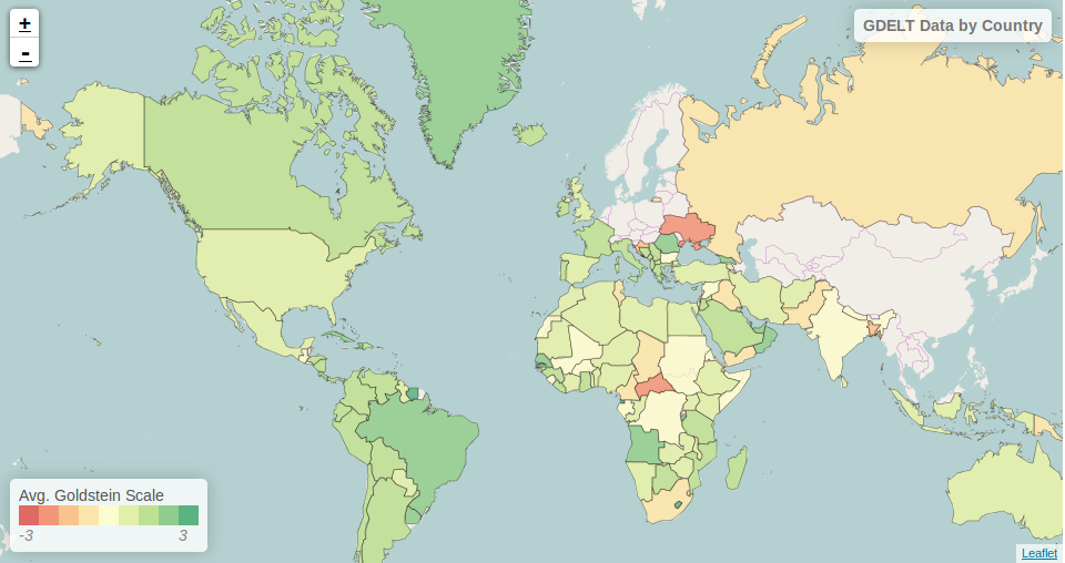
The final result of the analysis described in this tutorial is found in the Jupyter notebook: _static/geomesa-examples-jupyter/shallow-join-gdelt.ipynb.
You can find a static render of this notebook on Github.